Introduction
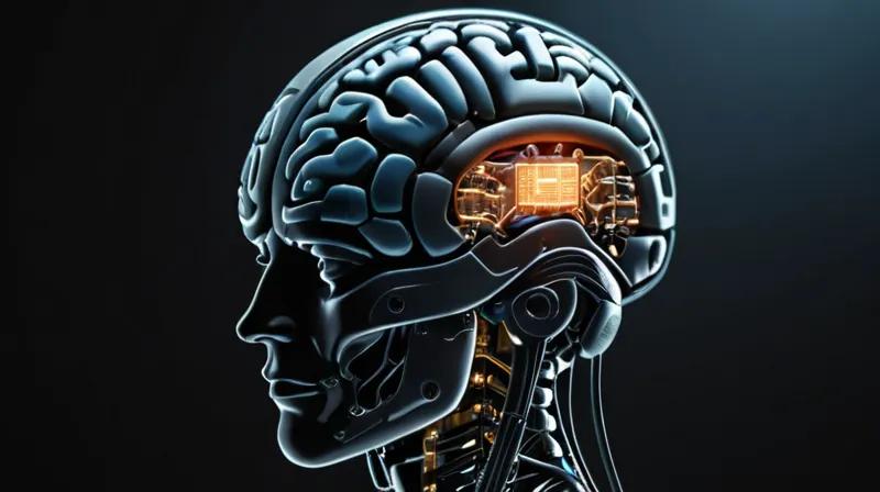
Brain-computer interfaces (BCIs) are rapidly evolving from science fiction to real-world applications. While China's approval of the NEO brain implant marks a significant milestone, the technology is also being explored in research labs and startups worldwide. In this tutorial, we'll explore how to interface with BCI data using Python, focusing on the fundamental concepts and practical implementation. This approach will help you understand how to work with neural signals, even without access to a physical implant.
Prerequisites
- Basic understanding of Python programming
- Familiarity with NumPy and Pandas for data manipulation
- Knowledge of signal processing concepts (filters, FFT)
- Python libraries: numpy, pandas, matplotlib, scipy
- Optional: Access to BCI data or simulation tools
Step-by-Step Instructions
1. Setting Up Your Environment
1.1 Install Required Libraries
We'll need several Python libraries to process and visualize BCI data. Start by installing them using pip:
pip install numpy pandas matplotlib scipy scikit-learnWhy this step? These libraries provide the foundation for handling neural data, performing signal processing, and creating visualizations essential for BCI research.
1.2 Create a Basic BCI Data Simulation
Since we don't have access to actual neural data, we'll simulate realistic BCI signals to understand how they're processed:
import numpy as np
import matplotlib.pyplot as plt
from scipy import signal

# Simulate neural data
fs = 250  # Sampling frequency
duration = 10  # seconds
t = np.linspace(0, duration, int(fs * duration))

# Create a simulated EEG signal with different frequency components
signal_1 = 5 * np.sin(2 * np.pi * 10 * t)  # 10 Hz component
signal_2 = 3 * np.sin(2 * np.pi * 50 * t)  # 50 Hz component
noise = np.random.normal(0, 0.5, len(t))

# Combine signals
neural_data = signal_1 + signal_2 + noise

# Plot the simulated data
plt.figure(figsize=(12, 4))
plt.plot(t[:200], neural_data[:200])
plt.title('Simulated Neural Signal')
plt.xlabel('Time (s)')
plt.ylabel('Amplitude')
plt.grid(True)
plt.show()
Why this step? Simulating data allows us to practice signal processing techniques without needing real hardware, helping us understand how BCI systems might process actual neural signals.
2. Signal Preprocessing
2.1 Apply Filtering to Remove Noise
Real neural signals are often contaminated with noise. We'll apply a bandpass filter to isolate relevant frequency bands:
# Design a bandpass filter (e.g., 8-30 Hz for motor imagery)
low = 8 / (fs / 2)
high = 30 / (fs / 2)
b, a = signal.butter(4, [low, high], btype='band')

# Apply the filter
filtered_signal = signal.filtfilt(b, a, neural_data)

# Plot original vs filtered signal
plt.figure(figsize=(12, 4))
plt.subplot(2, 1, 1)
plt.plot(t[:200], neural_data[:200])
plt.title('Original Signal')
plt.ylabel('Amplitude')

plt.subplot(2, 1, 2)
plt.plot(t[:200], filtered_signal[:200])
plt.title('Filtered Signal')
plt.xlabel('Time (s)')
plt.ylabel('Amplitude')
plt.tight_layout()
plt.show()
Why this step? Filtering is crucial in BCI systems to isolate meaningful neural activity from noise, which is essential for accurate brain decoding.
2.2 Compute Power Spectral Density
Understanding the frequency content of neural signals helps in identifying relevant brain activity:
# Compute power spectral density
frequencies, psd = signal.welch(filtered_signal, fs, nperseg=256)

# Plot PSD
plt.figure(figsize=(10, 4))
plt.semilogy(frequencies, psd)
plt.title('Power Spectral Density')
plt.xlabel('Frequency (Hz)')
plt.ylabel('Power Spectral Density')
plt.grid(True)
plt.show()
Why this step? PSD analysis helps identify dominant frequencies in neural signals, which can be used to classify different brain states or intentions.
3. Feature Extraction
3.1 Extract Time-Frequency Features
BCI systems often extract features from both time and frequency domains:
# Extract time-domain features
mean_val = np.mean(filtered_signal)
std_val = np.std(filtered_signal)
max_val = np.max(filtered_signal)
min_val = np.min(filtered_signal)

# Extract frequency-domain features
peak_freq = frequencies[np.argmax(psd)]
band_power = np.sum(psd[(frequencies >= 8) & (frequencies <= 30)])

# Display features
features = {
    'mean': mean_val,
    'std': std_val,
    'max': max_val,
    'min': min_val,
    'peak_frequency': peak_freq,
    'band_power': band_power
}

print("Extracted Features:")
for key, value in features.items():
    print(f"{key}: {value:.2f}")
Why this step? Feature extraction is a critical step in BCI systems, where raw neural signals are transformed into meaningful data that can be used for classification or control.
3.2 Implement Common Spatial Patterns (CSP)
CSP is a widely used technique in BCIs for extracting discriminative features:
# Simulate two different signal classes
signal_class_1 = 5 * np.sin(2 * np.pi * 10 * t) + np.random.normal(0, 0.5, len(t))
signal_class_2 = 3 * np.sin(2 * np.pi * 20 * t) + np.random.normal(0, 0.5, len(t))

# Simple CSP-like feature extraction
# This is a simplified version - real CSP requires more complex matrix operations
features_1 = np.abs(np.fft.fft(signal_class_1))[:len(t)//2]
features_2 = np.abs(np.fft.fft(signal_class_2))[:len(t)//2]

# Plot the features
plt.figure(figsize=(10, 4))
plt.plot(features_1, label='Class 1')
plt.plot(features_2, label='Class 2')
plt.title('Simplified CSP Features')
plt.xlabel('Frequency Bin')
plt.ylabel('Magnitude')
plt.legend()
plt.grid(True)
plt.show()
Why this step? CSP helps identify spatial patterns in neural signals that are most informative for distinguishing between different brain states or intentions.
4. Classification and Control
4.1 Implement Simple Classifier
With extracted features, we can classify different brain states:
# Create a simple classifier using scikit-learn
from sklearn.ensemble import RandomForestClassifier
from sklearn.model_selection import train_test_split

# Generate synthetic dataset
X = np.array([list(features.values()) for _ in range(100)])
# Create labels (0 for class 1, 1 for class 2)
Y = np.random.randint(0, 2, 100)

# Split data
X_train, X_test, y_train, y_test = train_test_split(X, Y, test_size=0.2, random_state=42)

# Train classifier
clf = RandomForestClassifier(n_estimators=100, random_state=42)
clf.fit(X_train, y_train)

# Predict
predictions = clf.predict(X_test)
accuracy = np.mean(predictions == y_test)
print(f"Classifier Accuracy: {accuracy:.2f}")
Why this step? Classification is the core function of BCI systems - determining what brain state or intention is represented by the neural signal.
4.2 Simulate Control Output
Finally, we'll simulate how these classifications might control an external device:
# Simulate control output based on classification
control_output = []
for pred in predictions:
    if pred == 0:
        control_output.append("Move Right")
    else:
        control_output.append("Move Left")

# Display results
print("Simulated Control Output:")
for i, output in enumerate(control_output[:10]):
    print(f"Sample {i+1}: {output}")
Why this step? This demonstrates how BCI systems translate neural signals into actionable commands, showing the practical application of brain decoding.
Summary
This tutorial provided an intermediate-level introduction to working with brain-computer interface technology. We covered simulating neural signals, preprocessing techniques, feature extraction, and simple classification methods. While we didn't use actual implant data, the concepts and code demonstrate how real BCI systems process neural information. Understanding these techniques is crucial for anyone interested in BCI development, neural engineering, or brain decoding research. As China's approval of commercial brain implants marks a significant step forward, this knowledge will be increasingly valuable in the rapidly advancing field of neural technology.