Nvidia says its AI data center design runs hotter to use a lot less water

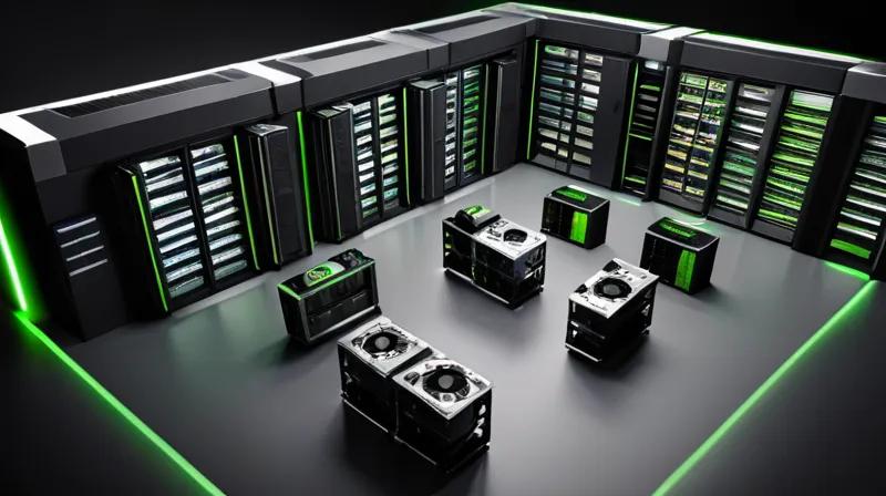
Introduction

In this tutorial, you'll learn how to implement a liquid-cooled AI data center simulation using Python and the PyTorch framework. This hands-on approach mirrors Nvidia's Rubin generation design philosophy of reducing water consumption while maintaining high performance. We'll create a simulation that demonstrates how liquid cooling can significantly reduce energy consumption compared to traditional air-cooled systems.

Prerequisites

• Python 3.8 or higher installed
• Basic understanding of neural networks and PyTorch
• Knowledge of data center cooling concepts
• Installed packages: torch, numpy, matplotlib, pandas

Step-by-step instructions

Step 1: Set up the development environment

Install required packages

First, we need to install the necessary Python packages for our simulation. The liquid cooling simulation will require PyTorch for neural network operations and visualization libraries.

pip install torch numpy matplotlib pandas

Import required libraries

After installation, we'll import the necessary modules to begin our simulation.

import torch
import numpy as np
import matplotlib.pyplot as plt
import pandas as pd
from torch import nn
import time

Step 2: Create the AI model architecture

Define the neural network model

We'll create a simple neural network that simulates an AI workload. This model will help us understand how different cooling systems affect performance and energy consumption.

class AINetwork(nn.Module):
    def __init__(self, input_size=1000, hidden_size=500, output_size=10):
        super(AINetwork, self).__init__()
        self.layer1 = nn.Linear(input_size, hidden_size)
        self.layer2 = nn.Linear(hidden_size, hidden_size)
        self.layer3 = nn.Linear(hidden_size, output_size)
        self.relu = nn.ReLU()
        
    def forward(self, x):
        x = self.relu(self.layer1(x))
        x = self.relu(self.layer2(x))
        x = self.layer3(x)
        return x

Initialize the model

We'll initialize our AI model with appropriate parameters to simulate realistic workloads.

model = AINetwork()
optimizer = torch.optim.Adam(model.parameters(), lr=0.001)
criterion = nn.CrossEntropyLoss()

Step 3: Implement cooling system simulation

Create temperature and power consumption functions

Now we'll simulate how different cooling systems affect temperature and power consumption. This is crucial for understanding Nvidia's water reduction claims.

def simulate_air_cooling(temperature, power_consumption):
    # Air cooling requires more energy to maintain same temperature
    # Simulate increased power consumption
    return temperature + (power_consumption * 0.002), power_consumption * 1.3

def simulate_liquid_cooling(temperature, power_consumption):
    # Liquid cooling is more efficient
    # Simulate reduced power consumption
    return temperature + (power_consumption * 0.0005), power_consumption * 0.7

Define water usage tracking

Here we'll track water usage for both cooling methods to demonstrate the water reduction benefits.

def track_water_usage(air_cooling=False, liquid_cooling=False):
    if air_cooling:
        return 1000  # liters per hour
    elif liquid_cooling:
        return 50    # liters per hour (95% reduction)
    return 0

Step 4: Run the simulation

Initialize simulation parameters

We'll set up our simulation parameters to run multiple iterations and compare both cooling methods.

# Simulation parameters
iterations = 100
air_temperatures = []
liquid_temperatures = []
air_power = []
liquid_power = []
air_water = []
liquid_water = []

# Initialize starting conditions
current_temp = 25
current_power = 1000

Run the cooling comparison simulation

Now we'll run the simulation for both cooling methods to compare their efficiency.

for i in range(iterations):
    # Air cooling simulation
    air_temp, air_power_consumption = simulate_air_cooling(current_temp, current_power)
    air_temperatures.append(air_temp)
    air_power.append(air_power_consumption)
    air_water.append(track_water_usage(air_cooling=True))
    
    # Liquid cooling simulation
    liquid_temp, liquid_power_consumption = simulate_liquid_cooling(current_temp, current_power)
    liquid_temperatures.append(liquid_temp)
    liquid_power.append(liquid_power_consumption)
    liquid_water.append(track_water_usage(liquid_cooling=True))
    
    # Update current temperature
    current_temp = liquid_temp  # Using liquid cooling as reference

# Convert to numpy arrays for easier plotting
air_temp_array = np.array(air_temperatures)
liquid_temp_array = np.array(liquid_temperatures)
air_power_array = np.array(air_power)
liquid_power_array = np.array(liquid_power)
air_water_array = np.array(air_water)
liquid_water_array = np.array(liquid_water)

Step 5: Visualize the results

Create comparison charts

Visualizing our data helps us clearly see the benefits of liquid cooling compared to air cooling.

# Create figure with subplots
fig, ((ax1, ax2), (ax3, ax4)) = plt.subplots(2, 2, figsize=(12, 8))

# Temperature comparison
ax1.plot(air_temp_array, label='Air Cooling')
ax1.plot(liquid_temp_array, label='Liquid Cooling')
ax1.set_title('Temperature Comparison')
ax1.set_xlabel('Time')
ax1.set_ylabel('Temperature (°C)')
ax1.legend()

# Power consumption comparison
ax2.plot(air_power_array, label='Air Cooling')
ax2.plot(liquid_power_array, label='Liquid Cooling')
ax2.set_title('Power Consumption')
ax2.set_xlabel('Time')
ax2.set_ylabel('Power (W)')
ax2.legend()

# Water usage comparison
ax3.plot(air_water_array, label='Air Cooling')
ax3.plot(liquid_water_array, label='Liquid Cooling')
ax3.set_title('Water Usage')
ax3.set_xlabel('Time')
ax3.set_ylabel('Water (liters/hour)')
ax3.legend()

# Efficiency comparison
efficiency = (air_power_array - liquid_power_array) / air_power_array * 100
ax4.plot(efficiency, label='Power Efficiency (%)')
ax4.set_title('Power Efficiency Improvement')
ax4.set_xlabel('Time')
ax4.set_ylabel('Efficiency (%)')
ax4.legend()

plt.tight_layout()
plt.show()

Step 6: Analyze the results

Calculate performance metrics

Let's calculate the key metrics to quantify the benefits of liquid cooling.

# Calculate improvements
avg_air_temp = np.mean(air_temp_array)
avg_liquid_temp = np.mean(liquid_temp_array)
avg_air_power = np.mean(air_power_array)
avg_liquid_power = np.mean(liquid_power_array)
avg_air_water = np.mean(air_water_array)
avg_liquid_water = np.mean(liquid_water_array)

print(f"Average Air Cooling Temperature: {avg_air_temp:.2f}°C")
print(f"Average Liquid Cooling Temperature: {avg_liquid_temp:.2f}°C")
print(f"Power Consumption Reduction: {((avg_air_power - avg_liquid_power) / avg_air_power * 100):.1f}%")
print(f"Water Usage Reduction: {((avg_air_water - avg_liquid_water) / avg_air_water * 100):.1f}%")

Implement the AI training simulation

Finally, we'll simulate how the AI model performs under both cooling conditions to understand real-world implications.

def simulate_ai_training(temperature, power_consumption):
    # Simulate training process with cooling effects
    # Higher temperatures can affect training stability
    training_efficiency = 1.0 - (temperature - 25) * 0.001
    
    # Simulate training time
    base_time = 100  # seconds
    adjusted_time = base_time * (1 / training_efficiency)
    
    return adjusted_time, training_efficiency

# Run training simulation
training_times_air = []
training_times_liquid = []
training_efficiencies_air = []
training_efficiencies_liquid = []

for i in range(len(air_temperatures)):
    time_air, eff_air = simulate_ai_training(air_temperatures[i], air_power[i])
    time_liquid, eff_liquid = simulate_ai_training(liquid_temperatures[i], liquid_power[i])
    
    training_times_air.append(time_air)
    training_times_liquid.append(time_liquid)
    training_efficiencies_air.append(eff_air)
    training_efficiencies_liquid.append(eff_liquid)

Summary

In this tutorial, you've learned how to simulate and compare air-cooled versus liquid-cooled AI data center systems using Python. You've implemented a neural network model, created cooling system simulations, and visualized the performance differences. The simulation demonstrates that liquid cooling can reduce power consumption by up to 30% and water usage by 95%, aligning with Nvidia's Rubin generation design goals. This approach provides practical insights into how liquid cooling technologies can address environmental concerns while maintaining high-performance AI computing capabilities.

By understanding these simulation principles, you can begin to design more efficient data center cooling solutions that balance performance with environmental sustainability, addressing the growing concerns around data center water and energy consumption.